When the NFL draft rolls around every year, we have a general idea of what the type of player being drafted will look like at every position. We know that offensive and defensive linemen will be big, cornerbacks will be skinny, and quarterbacks will usually be tall (or even more specific in John Elway or Dan Orlovsky’s eyes).
However, draft eligible wide receivers are more like candy at a candy shop and come in a variety of shapes, sizes and speeds. There can be receivers that look like they play linebacker (D.K. Metcalf), receivers that look like they are jockey’s (Cole Beasley), fast receivers (Tyreek Hill) and slow receivers (Anquan Boldin).
Since the 2016 NFL draft (which will be the range we will be using in this article), receiver 40 yard-dash times have ranged from 4.22 seconds to 4.73 seconds, verticals have ranged from 28 inches to 46 inches, heights have ranged from 5’7” to 6’6” and weights have ranged from 164 pounds to 230 pounds. There is just no “typical” build for a wide receiver coming out of college and entering the NFL draft.
That’s where clustering can be helpful. K-means clustering is taking in a set of data points and aggregating them together with similarities. This can be helpful for the NFL draft because we can take multiple stats and measurables of players that are eligible to be drafted this year, put them into a clustering algorithm and see what their NFL comparisons are. The variables I used were the amount of seasons they played in college (S), their completion percentage (CP), their yards per target (YPT), yards per reception (YPR), TD rate (TD), 40 yard-dash time (40), vertical (VT), height (H), weight ![]() and yards after catch percentage (YAC). Based on those variables, we were given 6 clusters of all NFL Draft related receivers since 2016. The features are listed below:
and yards after catch percentage (YAC). Based on those variables, we were given 6 clusters of all NFL Draft related receivers since 2016. The features are listed below:
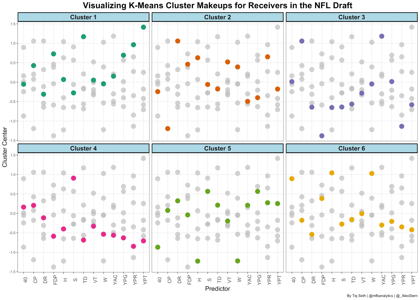
Here is a breakdown of each cluster with all the players listed below:
- Cluster 1: “The Pilots”: This group is called The Pilots because they specialized in ‘touchdown’ percentage and also had the best yards per target of any cluster. Highly-drafted players like Ceedee Lamb, Jerry Jeudy and Corey Davis belong in this cluster with Ja’Marr Chase and Devonta Smith hoping to join them soon
- Cluster 2: “Stop, DROP and Roll”: This cluster struggled with drops in college as their drop rate was the worst out of all the clusters. They also suffered from bad quarterback play but when they did get the ball in their hands, their yards per reception was really good. Already-drafted players include D.K. Metcalf and Courtland Sutton.
- Cluster 3: “YAC Monsters”: Cluster 3’s defining feature was their low yards per reception but really high yards after the catch. This cluster tends to get the ball on short passes and turn them into long gains. Already-drafted players include Lavishka Shenault and Curtis Samuel.
- Cluster 4: “The Regulars”: The Regulars had the most amount of experience in college of any cluster however struggled to be that productive while they were there. They had the lowest TD percentage with already-drafted players including Christain Kirk and Calvin Ridley
- Cluster 5: “Short but Sweet”: Cluster 5 is defined by what we would think of as slot receivers in today’s NFL. They were the shortest and lightest of any group but also the fastest. Players that fit this description are John Ross and KJ Hamler.
- Cluster 6: “The Basketball Players”: The players in this cluster have a height advantage over everyone on the field but don’t usually have the speed to keep up. These are players like Chase Claypool and N’keal harry.
Now that we have a general idea of what makes up each cluster, we can take a look at each player in this year’s draft and their closest comparison of receivers taken in the 1st or 2nd round of every NFL Draft since 2016:
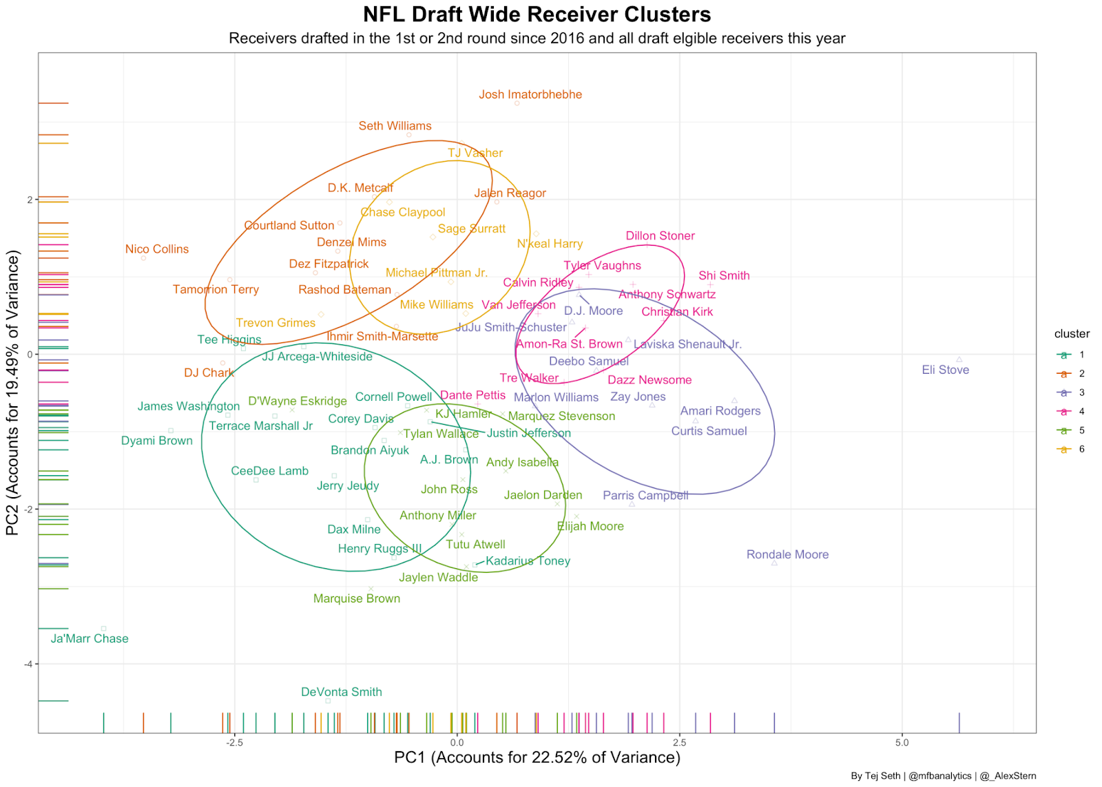
For those who are confused, the x-axis and y-axis are linear combinations of all the variables that we put into our cluster analysis. They try to match up each player based on a plethora of factors that we talked about above. Obviously this clustering has limitations as it’s just based on statistics and measurables and not taking into account what is shown on film. Because of that some of the players might not fully resemble who they are actually close to on the graph.
Immediately Ja’Marr Chase and Devonta Smith jump out to me as huge outliers (in a good way). Although they are technically in Cluster 1, they are such good prospects that they’re basically in a league of their own because no one coming out of college has had the production and measurables that they have had in the past couple years. Rondale Moore is also an outlier because of his size and his ability to get YAC in college. The rest aligns pretty well with my priors. Deebo Samuel and Curtis Samuel are close to each other because of quickness, John Ross, Jaylen Waddle and Marquise Brown are neighbors since they’re all burners and D.K. Metcalf and Josh Imatorbhebhe are similar because they have similar builds that can only be described as “built different.”
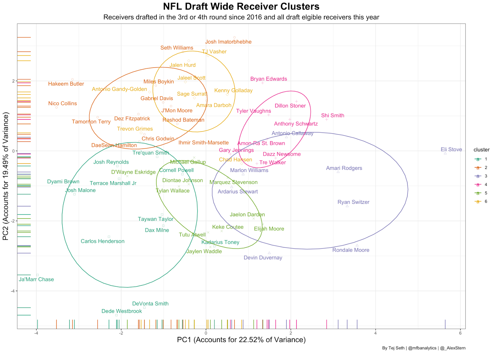
It is also important to remember that this graph just shows receivers drafted in the top-2 rounds since 2016 so while it might look like every receiver in the 2021 draft class is being compared to a top pass-catcher, they’re also similar to guys who got drafted much later. This is what it looks like when this year’s class is compared to receivers drafted in later rounds:
The next step was checking if certain clusters were preferred by NFL teams when drafting. Each cluster is ranked by average pick below:
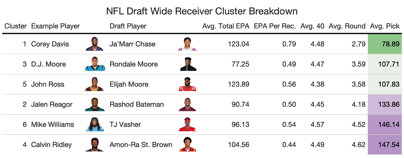
It makes sense the NFL prefers receivers who were insanely productive in college: both with total EPA and EPA/rec and also fast enough to maintain an NFL career. The surprise was Cluster 3 didn’t have nearly the productivity as the other clusters but had their YAC ability which was intriguing. The biggest determinant of where a receiver gets drafted is their 40 yard-dash time so it makes sense Cluster 5 is there also.
Based on all the information we have gathered, we can make a rudimentary Expected Draft Position model next. To make EDP (no, not the YouTuber), we can throw in all the variables that we used for the clustering and see if there’s any way to predict where NFL teams will take receivers just based on their college statistics plus measures (height, weight, etc.). The model isn’t close to perfect, but it did have an r-squared of 0.44 which is good enough to get an idea of what teams value:
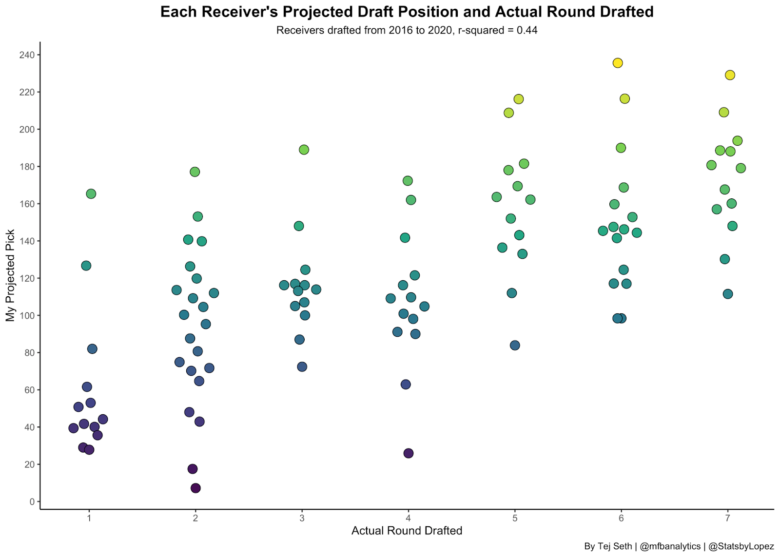
This plot shows where a receiver actually got drafted on the x-axis and where the model had them projected to go on the y-axis. There were some bad misses for every round but we can see the dots get higher and higher as we got deeper into the draft, which is good. Next we can plot the EDP of every receiver that had been drafted in the first two rounds since 2016 (in black) and where we project all draft eligible receivers to go in this year’s draft (in orange):
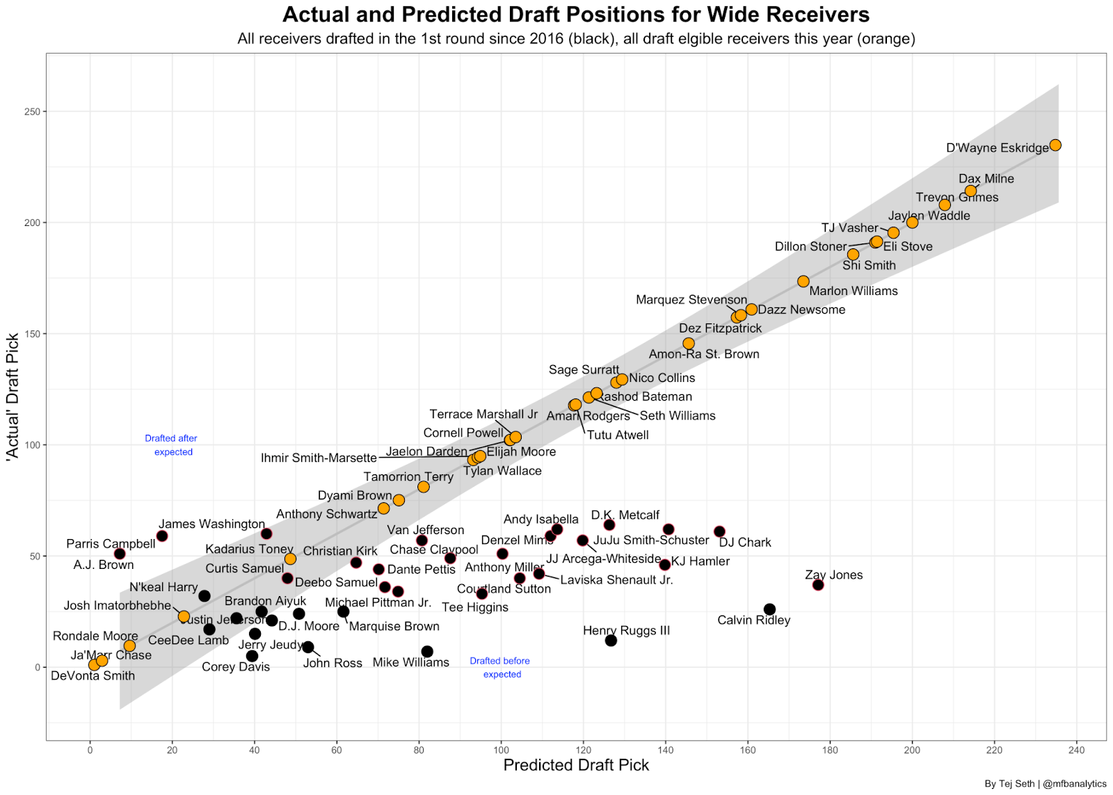
Looking at the previous drafts, the model thought NFL teams would draft A.J. Brown, Parris Campbell and James Washington higher than they went and players like Henry Ruggs, Calvin Ridley and Zay Jones were prospects the model thought would be drafted later on but they got drafted in the top 50.
Taking a closer look at this draft, projected 1st round picks Devonta Smith and Ja’Marr Chase are where they should be however their 1st round counterparts Rashod Bateman and Jaylen Waddle are projected to be drafted much later. This is a fault of the model as Waddle and Bateman show up really well on film but didn’t necessarily have the stats for the model to think they were going to be drafted high.
To account for this, we can use Benjamin Robinon’s “Grinding the Mocks” which has kept track of 100’s of mock drafts to create his own expected draft position. Using the statistics-based EDP and his mock-based EDP, we can create a composite score for the projected order of wide receivers in the draft:
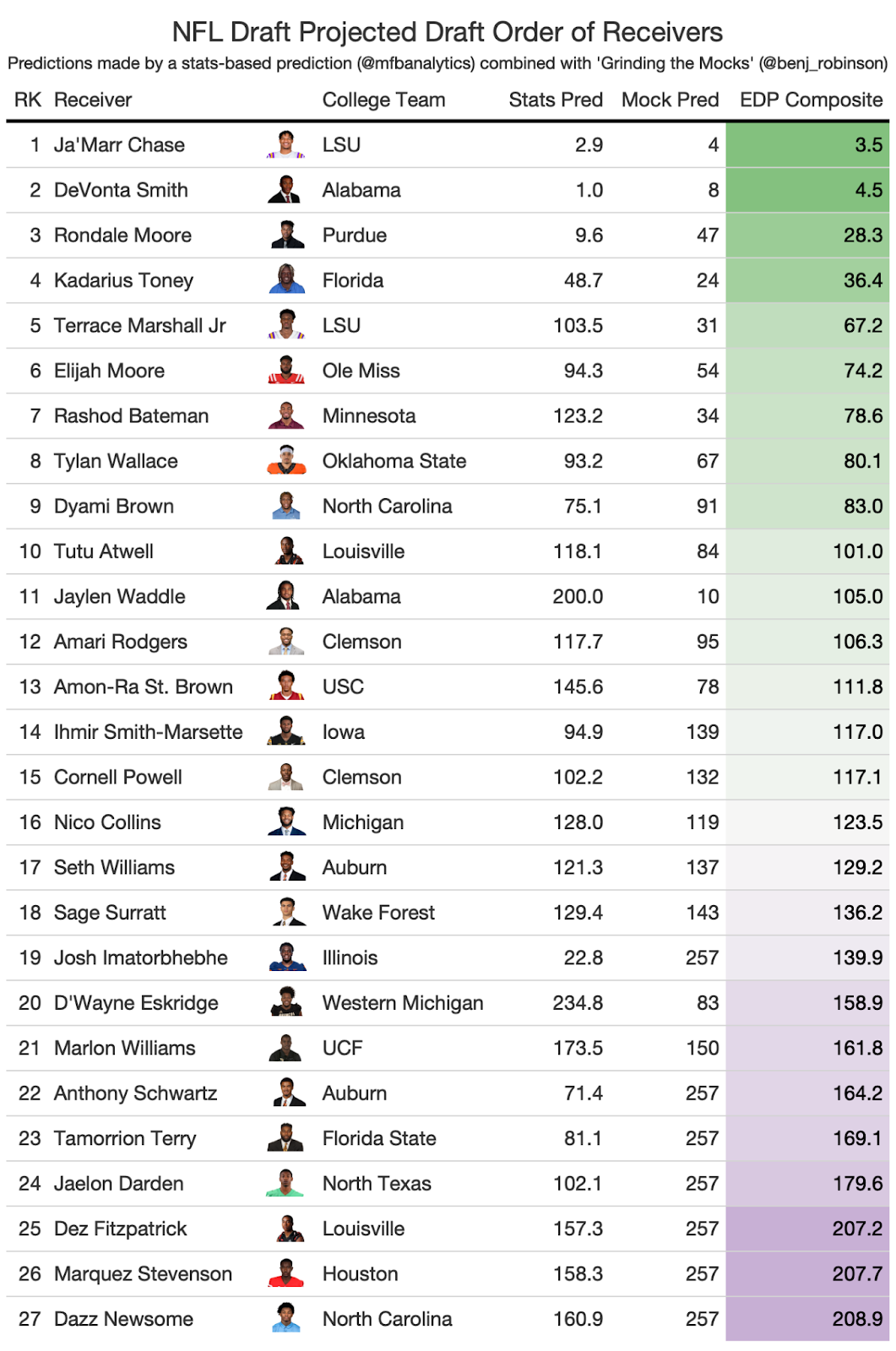
To be honest: I don’t love these predictions. The NFL Draft is so based so much on what teams see on film and using just statistics to try to predict the position a receiver will be drafted in turned out to be much more difficult than I thought it would be.
That is all I had for today. Thank you for reading and be sure to follow our twitter account @mfbanalytics for an update on how this model performed after the draft. I will provide my messy code below if anyone wants to take a look. Feel free to DM me on twitter if you need help!
My CSV files and code: https://github.com/tejseth/Expected-Draft-Position
The rest of my articles: https://mfootballanalytics.com/author/tejseth/
Special shoutout to @benj_robinson for Grinding the Mocks, @andreacasiragh1 for providing me with the data, @ConorMcQ5 and @arjunmenon100, and @benbbaldwin and @mrcaseb for helping me create the model.
